Tutorial

The Inflation package contains implementations of the inflation technique for causal compatibility. It supports the linear-programming technique of [1], that is used for compatibility with classical and theory-independent models, and the semidefinite-programming method of [2], that is used for compatibility with classical and quantum models. It also supports hybrid scenarios where the systems distributed by different sources are described by different physical theories. The implementation of Inflation follows an object-oriented design. The workflow comprises of three main steps:

• Encode the causal scenario and desired inflation as an instance of InflationProblem.

• Generate the associated optimization problem for classical, quantum, or theory-independent inflation, via InflationLP or InflationSDP depending on the goal.

• Export the problem to a file and/or solve it.

We will now go through the steps above in more detail. This tutorial is available on the documentation webpage and it can also be downloaded as a ready-to-run Jupyter Notebook from the GitHub repository. If already familiar with inflation, the quickest way to get started is to run some examples from the Examples section, which can also be downloaded as a Jupyter Notebook.

We start by importing everything that we will need:

from inflation import InflationProblem, InflationLP, InflationSDP
import numpy as np

Encoding the inflation problem

The first object of interest is InflationProblem. When instantiating it, we pass all the relevant information about the causal scenario and the type of inflation we want to perform.

Basics of causal diagrams

Causal relationships are encoded through a Bayesian Directed Acyclic Graph, or DAG for short. The nodes of the graph represent random variables, which can be either observable (visible) or unobservable (hidden). Directed arrows encode causal influences between nodes. Arrows point from parent nodes to the nodes causally influenced by them, called children nodes. The acyclicity property avoids the presence of causal loops.

For applications to physics, another class of random variables is often considered called “settings”. These correspond to observable variables on whose outcome we condition in order to obtain the observed data. For example, this might correspond to measuring one property of a system versus another in an experiment. Furthermore, in physics we also have sources generating quantum correlations. These are modeled through the presence of quantum unobservable variables, which represent quantum systems. Arrows going into a quantum node represent controlling the corresponding quantum system. Arrows going out of the quantum node represent the children of the quantum node generating statistics by measuring the quantum system.

The tripartite line network

As an example, let us consider the tripartite line, or “bilocality scenario” [3], which corresponds to the scenario where three space-like separated parties (\(A\), \(B\) and \(C\)) measure two physical systems \(\rho_{AB}\), \(\rho_{BC}\) that never interacted in the past. The subindex of the systems indicates which parties have access to and can measure that state. This is a simple scenario where, for instance, entanglement swapping [4] can be performed, which is at the heart of the quantum teleportation protocol [5]. The corresponding DAG is:

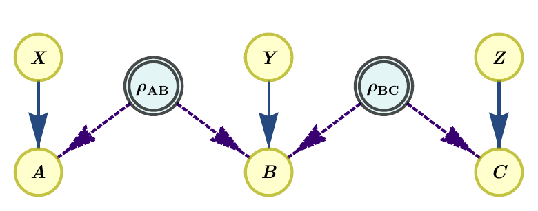
We have three observed random variables, \(A\), \(B\) and \(C\), two latent variables \(\rho_{AB}\) and \(\rho_{BC}\) denoting the physical systems sent to the parties, and three setting variables, \(X\), \(Y\) and \(Z\). We assume all observed variables have cardinality 2, i.e., \(a,b,c,x,y,z \in \{0, 1\}\), where lower case denotes specific values that the random variables (in upper case) can take. In this causal scenario, correlations are generated by measuring the systems conditioned on the values of the settings. These correlations are encoded in the joint probability distribution \(p(a,b,c|x,y,z)\). Notice that the probability distribution is not conditioned on \(\rho_{AB}\), \(\rho_{BC}\) as they are latent variables.

Causal compatibility and inflation

One of the fundamental questions to ask is whether a given a probability distribution \(p(a,b,c|x,y,z)\) is compatible with a given causal scenario. The challenge in answering this question comes from the assumption of statistical independence of the sources \(\rho_{AB}\) and \(\rho_{BC}\). Inflation techniques are general methods that can give an answer to this question by relaxing the independence constraint. Let us consider an inflation of the bilocal scenario where we take two copies of each source, as in the following figure:

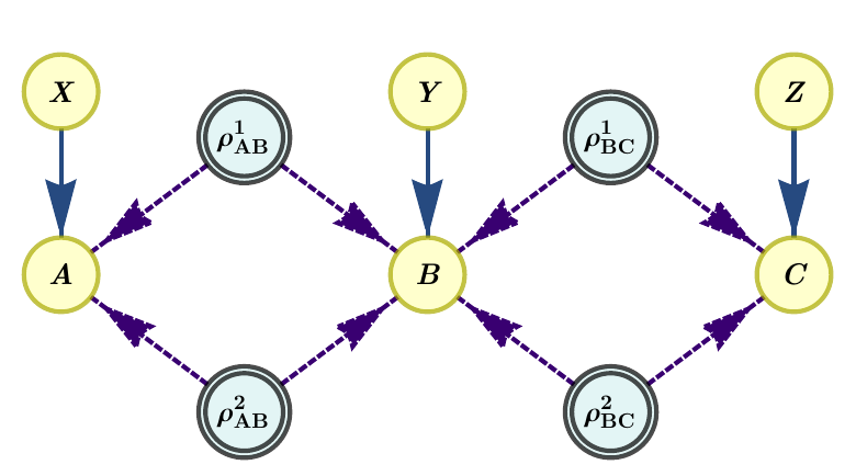
Depending on the nature of the systems distributed by the sources, the parties will be able to perform different operations on them. If the systems are classical, the parties can clone them and feed them to copies of their measurement devices. If they are quantum, the systems cannot be cloned, but the parties can choose on which copies of the systems to perform their measurements. If they are general physical states, then the parties can only use complete copies of the measurement devices and just feed one copy of each of the corresponding systems to each of them. These different operations are exploited to relax the independence conditions to symmetry conditions, that give rise to problems that can be formulated in terms of linear programming (in the case of classical and theory-independent models [1]) or semidefinite programming (in the case of quantum models [2]) using the NPA hierarchy [6]. These symmetries arise from the extra sources in the inflated graph being copies of the original sources, e.g., \(\rho_{AB}{=}\rho_{AB}^1{=}\rho_{AB}^2\). If the feasible region of the LP or SDP is empty, then we can conclude that the distribution \(p(a,b,c|x,y,z)\) is incompatible with the particular realization in the causal graph, and furthermore, we get an analytical certificate. This certificate can be understood as a Bell-like inequality for the class of models considered in the particular network. For more details, see [1] and [2].

Creating an instance of InflationProblem

The first step in using Inflation is encoding the scenario to be analyzed. This is done by providing a description of the target DAG, as well as the cardinalities of its visible variables (and optionally a number of possible measurement settings for each one). Also, one must specify the inflation that shall be constructed, by providing the amount of copies of each of the latent variables in the DAG that the inflation will contain. All this information is passed to an instance of InflationProblem as follows:

InfProb = InflationProblem(dag={"h1": ["v1", "v2"],
                                "h2": ["v2", "v3"]},
                           outcomes_per_party=[2, 2, 2],
                           settings_per_party=[2, 2, 2],
                           inflation_level_per_source=[2, 2])

The DAG is written as a dictionary where the keys are parent nodes, and the values are lists of the corresponding children nodes. In outcomes_per_party and settings_per_party we specify the cardinalities of visible nodes. The parameter inflation_level_per_source determines how many copies of the quantum sources we consider in the inflated graph. Another important argument is classical_sources, that allows to determine which of the sources will be assumed to be classical. This will be important for problems involving compatibility with classical causal models, and with hybrid models.

Internally, Inflation handles scenarios as networks, which are bipartite DAGs with one layer of visible nodes (the outcomes) and another layer of both visible (the settings) and latent (the sources) nodes. If the DAG contains visible-to-visible connections (such as in the instrumental scenario [7]), InflationProblem automatically finds an equivalent network and keeps track of the correspondence when setting values and bounds.

Generating the relaxation: example with quantum compatibility

For the sake of simplicity, we are going to consider the specific problem of compatibility with quantum models in the bilocality scenario. For examples of other types of inflations, see the end of this page.

Once the scenario is set up, the next step is generating the associated characterization of distributions admitting a realization in the inflation. In order to consider compatibility with quantum models, one needs to use the object InflationSDP, which generates the corresponding characterizations as semidefinite programs. InflationSDP is an object that takes as input an instance of InflationProblem:

InfSDP = InflationSDP(InfProb)

The first main method, InflationSDP.generate_relaxation generates the SDP relaxation of the chosen inflation.

InfSDP.generate_relaxation('npa2')

In the above example, we have chosen NPA hierarchy level 2. For the meaning of these levels, see [6]. For other hierarchies that we support, see the documentation of InflationSDP.generate_relaxation, or the Examples section. The important thing to know is that the higher the hierarchy level, the tighter is the SDP relaxation (at the cost of needing more computational resources).

Running a feasibility problem

If we have a specific distribution in mind, we can test whether such distribution can be generated in a certain causal structure. We can consider for the example the 2PR distribution, which is defined as

\[P_{\text{2PR}}(abc|xyz) := \frac{1+ (-1)^{a+b+c+xy+yz}}{8}\]

and it is known to be incompatible with the quantum tripartite line scenario. We impose the corresponding constraints on the semidefinite program with InflationSDP.set_distribution and then we attempt to solve the program:

P_2PR = np.zeros((2,2,2,2,2,2))

for a,b,c,x,y,z in np.ndindex((2,2,2,2,2,2)):
    P_2PR[a,b,c,x,y,z] = (1 + (-1)**(a + b + c + x*y + y*z))/8

InfSDP.set_distribution(P_2PR)
InfSDP.solve()
InfSDP.status

'infeasible'

The problem status is reported as infeasible, therefore this serves as a proof that the 2PR distribution cannot be generated by measuring two independent quantum states, \(\rho_{AB}\) and \(\rho_{BC}\), in the tripartite line scenario.

We can also export the problem with InflationSDP.write_to_file method and run it with another solver. Currently, supported formats are .mat for MATLAB, .dat-s for various solvers and platforms (for instance, Yalmip), and .csv for a human-readable output.

Running an optimisation problem

Inflation also supports the optimization of objective functions over the sets of distributions compatible with a given inflation. This is useful for finding bounds of Bell operators in complex multipartite scenarios. For example, we can calculate upper bounds on the value of the Mermin inequality, defined as:

\[\text{Mermin} = \langle A_1 B_0 C_0 \rangle + \langle A_0 B_1 C_0 \rangle + \langle A_0 B_0 C_1 \rangle - \langle A_1 B_1 C_1 \rangle\]

over the tripartite line scenario:

InfSDP.generate_relaxation('npa2')

mmnts = InfSDP.measurements
A0, B0, C0, A1, B1, C1 = (1-2*mmnts[party][0][setting][0]
                          for setting in range(2)
                          for party in range(3))

InfSDP.set_objective(A1*B0*C0 + A0*B1*C0 + A0*B0*C1 - A1*B1*C1)
InfSDP.solve()

InfSDP.objective_value

3.4615797540545383

We get that the value of the Mermin Bell operator cannot achieve a value greater than \(\approx 3.4616\) in the quantum tripartite line scenario. This is less than the algebraic value of \(4\) which is achievable when using tripartite quantum states distributed to \(A\), \(B\) and \(C\).

Inflations for different physical models

The example discussed above deals with considering quantum models of the distributions of interest. However, it is also possible to consider classical models, and theory-independent (also known as non-signaling) models of physical systems. In order to characterize these, one needs to use the object InflationLP, which generates the corresponding characterizations as linear programs. The usage of InflationLP is similar to that of InflationSDP. Below we show an example of how to use both objects to bound the maximum visibility for which the Popoescu-Rohrlich box admits classical, quantum, and theory-independent models. This is, we will consider how large the parameter \(v\) in the distribution

\[P_v(a,b|x,y) = \frac14 \left[ 1 + v(-1)^{a+b+xy}\right]\]

can achieve in different models of physical systems.

In order to do this we will use the auxiliary function max_within_feasible, which is explained in more detail in Example 5 in the Examples page.

from inflation import max_within_feasible
from sympy import Symbol
import numpy as np

def PR(v):
    p = np.zeros((2, 2, 2, 2), dtype="object")
    for a,b,x,y in np.ndindex((2,2,2,2)):
        p[a,b,x,y] = (1 + v*(-1)**(a+b+x*y)) / 4
    return p

# The different scenarios
bell      = {"l": ["A", "B"]}
outcomes  = [2, 2]
settings  = [2, 2]
inflation = [2]

# Classical
classicalScenario = InflationProblem(dag=bell,
                                     outcomes_per_party=outcomes,
                                     settings_per_party=settings,
                                     inflation_level_per_source=inflation,
                                     classical_sources='all')

# Quantum and theory-independent
nonclassicalScenario = InflationProblem(dag=bell,
                                        outcomes_per_party=outcomes,
                                        settings_per_party=settings,
                                        inflation_level_per_source=inflation)

# The numerical characterizations
classical    = InflationLP(classicalScenario)
quantum      = InflationSDP(nonclassicalScenario)
quantum.generate_relaxation('npa1')
nonsignaling = InflationLP(nonclassicalScenario)

for problem, name in [[classical, 'classical'],
                      [quantum, 'quantum'],
                      [nonsignaling, 'nonsignaling']]:
    problem.set_distribution(PR(Symbol("v")))
    v = max_within_feasible(problem, problem.known_moments, "bisection",
                            bounds=[0, 1+1e-5])     # For numerical stability
    print(f"(Upper bound to) maximum v in {name} teories: {v}")

(Upper bound to) maximum v in classical teories: 0.4999439642333985
(Upper bound to) maximum v in quantum teories: 0.7070993560791016
(Upper bound to) maximum v in nonsignaling teories: 0.9999489642333985

For more examples and features of the package, check out the Examples section.

References

[1] E. Wolfe, R. W. Spekkens, and T. Fritz, The inflation technique for causal inference with latent variables, J. Causal Inference 7, 20170020 (2019), arXiv:1609.00672.

[2] E. Wolfe, A. Pozas-Kerstjens, M. Grinberg, D. Rosset, A. Acín, and Miguel Navascués, Quantum inflation: A general approach to quantum causal compatibility, Phys. Rev. X 11, 021043 (2021), arXiv:1909.10519.

[3] C. Branciard, D. Rosset, N. Gisin, and S. Pironio, Bilocal versus non-bilocal correlations in entanglement swapping experiments, Phys. Rev. A 85, 032119 (2012), arXiv:1112.4502.

[4] M. Żukowski, A. Zeilinger, M. A. Horne, and A. K. Ekert, “Event-ready-detectors” Bell experiment via entanglement swapping. Phys. Rev. Lett. 71, 4287.

[5] C. H. Bennett, G. Brassard, C. Crépeau, R. Jozsa, A. Peres, and W. K. Wootters, Teleporting an unknown quantum state via dual classical and Einstein-Podolsky-Rosen channels, Phys. Rev. Lett. 70, 1895 (1993).

[6] M. Navascués, S. Pironio, and A. Acín, A convergent hierarchy of semidefinite programs characterizing the set of quantum correlations, New J. Phys. 10 073013, arXiv:0803.4290.

[7] T. Van Himbeeck, J. Bohr Brask, S. Pironio, R. Ramanathan, A. Belén Sainz, and E. Wolfe, Quantum violations in the Instrumental scenario and their relations to the Bell scenario, Quantum 3, 186 (2019), arXiv:1804.04119.